Linear regression analysis is a widely used statistical technique used to explore relationships among continuous variables. In addition, this technique can be applied to categorical variables through the use of dummy variables.
There are many situations where linear regression is useful. For instance,
- A market researcher can use regression to determine which one of several media markets is the best on which to spend their advertising dollars;
- In business, regression can be used to predict a competitive salary offer for a programmer with a given number of years of experience;
- In Major League Baseball, regression can be used to predict the salaries of free agents;
- In social science research, regression can predict a wide range of phenomena—from economic performance to college enrollment.
1 Simple Linear Regression
Simple linear regression refers to the statistical relationship between a dependent continuous variable, say y, and a single independent continuous variable, say x. This relationship takes the form of an equation that lets us predict values of y given values of x. Regression equations are useful for estimating new data values or exploring “what if” questions.
As an example of simple linear regression, suppose you survey a group of workers and notice that those who have more years of education tend to have received higher starting salaries when they began working. A linear regression analysis allows you to quantify the relationship between starting salary and years of education through an equation that you can then use to make predictions about starting salaries for other individuals.
Linear regression analysis allows you to (1) determine whether one or more continuous (independent) variables can effectively predict the values of an outcome (dependent) variable and (2) quantify the impact that each independent variable has on that outcome variable.
The relationship between a dependent variable and a single independent variable can be visualized using a scatter plot, as shown in Figure 1, below. The figure shows a set of data points along with the “best-fit” line that results from a regression analysis of that data.
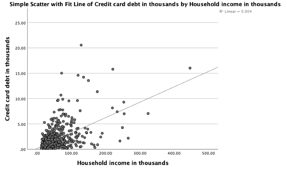
Figure 1: A scatter plot showing the relationship between credit card debt (in thousands) and household income (also in thousands)
The line is represented in general form by the equation
where b is the slope (the change in y per unit change in x) and a is the intercept (the value of y when x is zero). People are usually more interested in the slope than in the intercept. Also, note that a and b depend on the unit of measurement of the variables and, as such, do not necessarily indicate anything about the strength of the relationship.
As you can see, the data points don’t necessarily fall on this line, so it’s important to evaluate how well the line actually represents the data. To determine this, we start by looking at the correlation between the x and y values, and calculating a correlation coefficient, r, to quantify this relationship. Because the correlation coefficient can take on negative values and we prefer to work with only positive values, we typically square it (r**2) and refer to it as R-squared. This quantity lies on a scale from 0 (no linear association) to 1 (perfect linear association), and can be interpreted as the proportion of variation in one variable that can be predicted from the other. Thus an R-squared of 0.5 indicates that you can account for 50% of the variance in one variable if you knew the values of the other variable. Think of this value as a measure of the improvement in your ability to predict one variable from the other (or others if there are multiple independent variables).
While R-squared provides a good starting point for determining how well your regression equation fits your data, a more rigorous way involves performing statistical tests to determine the statistical significance of the relationship. A relationship that is statistically significant means that your regression equation can reliably make predictions given new values of the independent variable. In other words, the predictions are more likely to be due to some factor of interest rather than random chance.
Referring to Figure 1, notice that many points fall near the line but some are quite a distance from it. For each point, the difference between the value of the dependent variable and the value predicted by the equation (the value on the line) is called the residual (also known as the error). Points above the line have positive residuals (the equation under-predicted them), those below the line have negative residuals (the equation over-predicted them), and those points falling on the line have a residual of zero (perfect prediction). Points having relatively large residuals are of interest because they represent instances where the prediction performed poorly. Outliers, or points far from the positions of the other points, are of interest in regression because they can exert a considerable influence on the equation (especially if the sample size is small).
Let’s apply linear regression analysis to an example in which household income is the independent (predictor) variable and credit card debt is the dependent variable. A standard linear regression analysis generates three tables depicting the relationship between the two variables. Here are several key points about the information appearing in those tables:
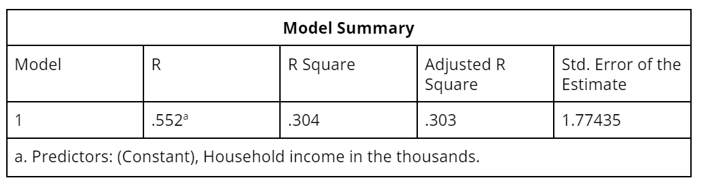
- The model summary table provides several measures of how well the model fits the data (see Table 1).
- As discussed above, R-squared, which can range from 0 to 1, is the correlation coefficient squared. It can be interpreted as the proportion of variance of the dependent measure that can be predicted from the independent variable(s).
- The adjusted R-squared represents a technical improvement over R-squared in that it explicitly adjusts for the number of predictor variables relative to the sample size. If the adjusted R-squared and R-squared differ dramatically, it is a sign that you have used too many predictor variables for the sample size.
- The standard error of the estimate is a measure of the standard deviation of the residuals. It represents the amount of variation that is not accounted for by the regression line on the scale of the dependent variable.
While the goodness-of-fit measures indicate how well you can expect the regression equation to predict the dependent variable, they do not tell whether there is a statistically significant relationship between the dependent and independent variable(s). For this, we turn to an analysis of variance (ANOVA) table, which presents technical summaries (i.e., sums of squares and mean square statistics) of the variation accounted for by the prediction equation (Table 2). The main goal is to determine whether there is a statistically significant (non-zero) linear relation between the dependent variable and the independent variable(s).
The significance (Sig.) column in the ANOVA table provides the probability that there is no relationship between the dependent and independent variable(s). A zero or nearly zero Sig. value means that the relationship is statistically significant and that you should further investigate the results of the regression coefficients appearing in the Coefficients table (Table 3).
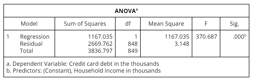
Table 2: ANOVA table showing sums of squares, mean squares, and the probability that there is no relationship between dependent and independent variables
The first column contains a list of the independent variables plus the intercept (constant). The intercept is the value of the dependent variable when the independent variable is 0—it is also a in the equation .
- The column labeled B contains the estimated regression coefficients you would use in a prediction equation. In this example, the coefficient for household income indicates that on average, each additional unit increase in household income is associated with an increase of 0.030 in credit card debt.
- The Std. Error column contains standard errors of the regression coefficients. The standard errors can be used to calculate a 95% confidence interval above and below the B coefficients. (This means that statistically, the true value of B will fall within this interval 95% of the time.)
- Betas are standardized regression coefficients used to judge the relative importance of each of several independent variables.
- The t statistics provide a significance test for each B coefficient, indicating which predictors are statistically significant.
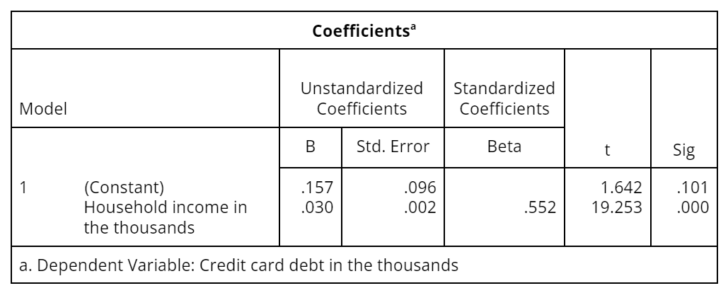
Table 3: A tabulation of statistical information for the coefficients in the regression model relating credit card debt to household income
2 Multiple Linear Regression
Regression involving more than one independent variable is called multiple linear regression and is a direct extension of simple linear regression. When running a multiple linear regression analysis you are again concerned with fitting a linear model to the data, determining whether any of the variables are significant predictors, and estimating the coefficients of the best-fitting prediction equation. In addition, you are interested in the relative importance of the independent variables in predicting the dependent measure.
Continuing with the previous example, we add age, years with current employer, and having previously defaulted as independent variables to the model, which now explains about 43% of the variance in credit card debt. This is a substantial increase in explanatory power from the 30% we were able to explain with just one predictor variable, namely household income.
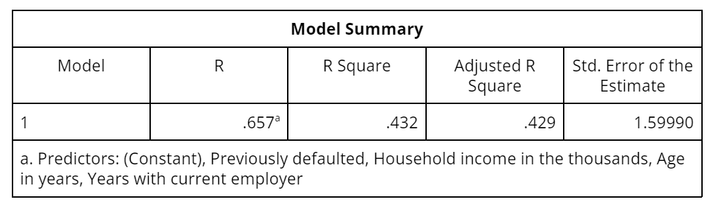
Table 4: The model summary table for a multiple linear regression
Not surprisingly, we still have a statistically significant model as shown in the ANOVA table Table 5).
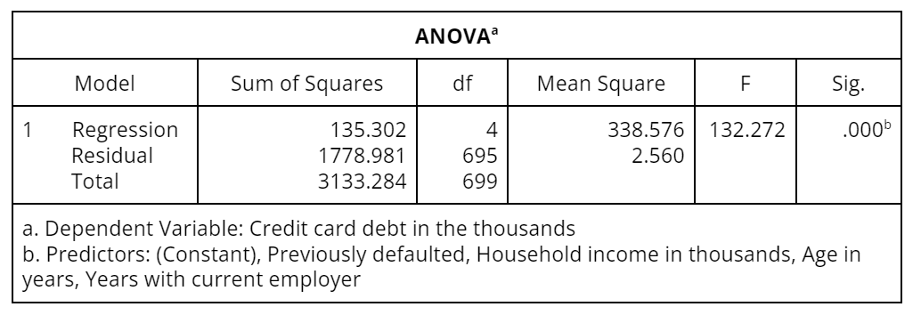
Table 5: ANOVA table showing sums of squares, mean squares, and the probability that there is no relationship between dependent and independent variables
Finally, we can see in Table 6 that all of the variables in the model are statistically significant except age, which means that we can remove this variable from the model. We can also see that household income is the most important predictor, followed by previous defaults, and then years with the current employer. We can use the regression equation that resulted from this analysis to predict someone’s credit card debt as follows:
Note that “previously defaulted” is a categorical variable, which is coded as a dummy variable in which “no” is 0 and “yes” is 1.
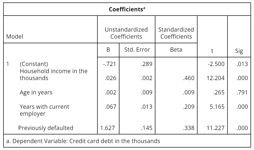
Table 6: A tabulation of statistical information for the coefficients in the regression model relating credit card debt to household income, age, years with employer, and previous defaults
3 Polynomials and Interaction Terms
This is an advanced and important topic. It is not true that linear regression can identify only linear relationships. It can handle curvilinear relationships as well if you know how to prepare the data. For instance, if you determined (through visual inspection) that income would predict credit card debt better with a quadratic relationship, you could do the following.
- Create a new variable consisting of income squared
- Add another coefficient corresponding to the new variable
It would look like this:
where = income and = income squared.
Another feature you might uncover through visual inspection is a pair of variables that interact. Here again the solution is to create a new variable. A good indicator that you have an interaction occurring is if the slopes of the regression lines for two groups (e.g., males and females) are different. In our example, this would suggest that the relationship between credit card debt and income is different for people that had previously defaulted on a loan than it is for people that had not previously defaulted on a loan (see Figure 2).
The resulting regression formula looks like this:
where = income and = previously defaulted. The interaction appears as the product .
If you fail to include the interaction term, the model will mathematically force the lines to be parallel and maintain the same “ gap” over the entire income range. Figure 2 makes it clear that this would not be accurate since the gap is clearly more severe at higher levels of income. Polynomials and interaction terms can seem tricky and abstract at first, but they are critical for understanding neural networks, which will be presented in a later module.
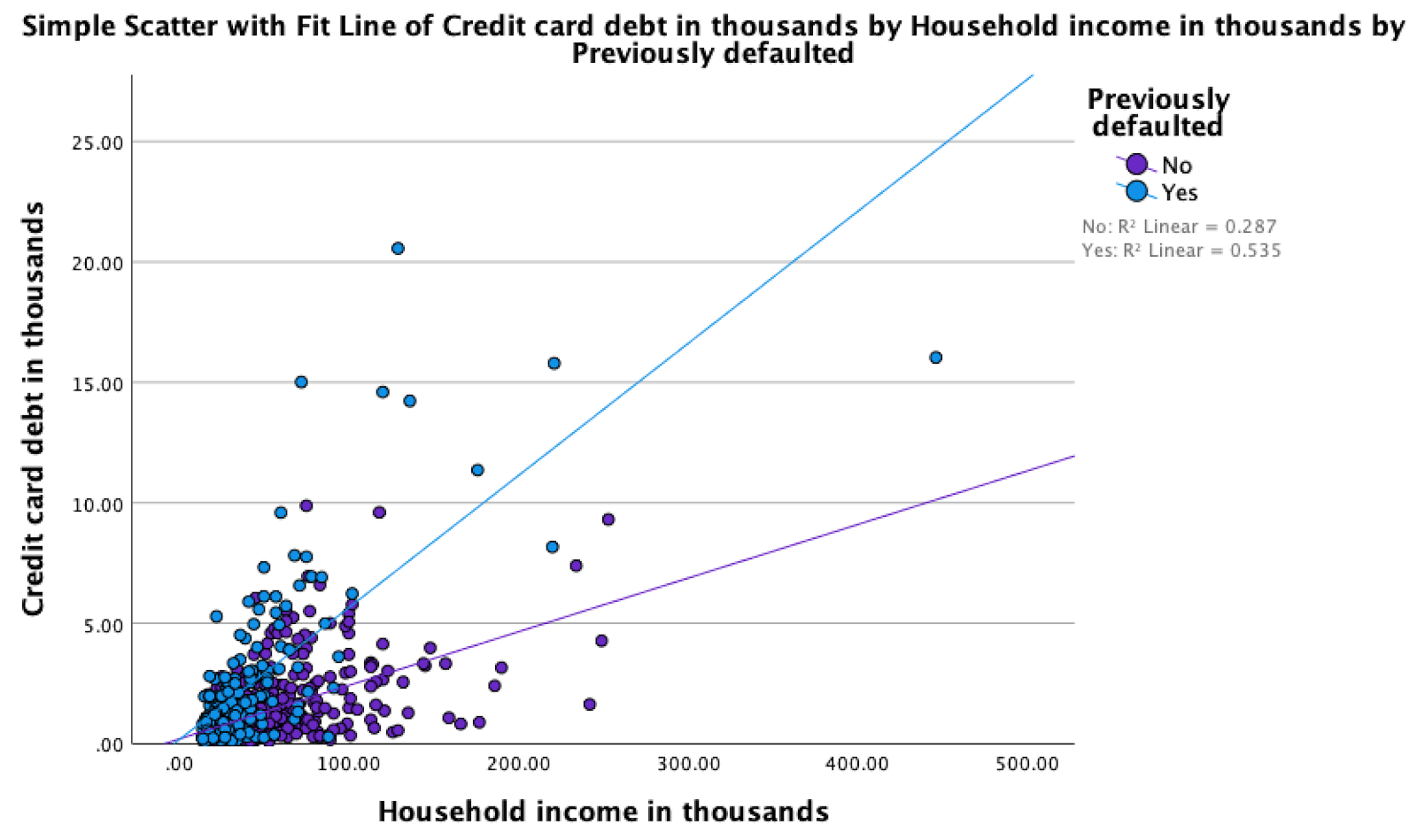
Figure 2: Differing linear regression line slopes for customers that had and had not previously defaulted on a loan