1 Introduction
Linear programming (LP) is a powerful tool to optimally solve a wide variety of business problems. Despite its power and widespread use, LP also comes with a few restrictive assumptions. Some of these assumptions can be removed or relaxed by using a slightly modified formulation of optimization problems, and the two assumptions that stand out in this front are:
- Divisibility: In LP, it is assumed that the solution (i.e., the values assigned to the decision variables) can be real/fractional numbers. We all know that many decision variables cannot have fractional values, such as the number of certain types of products to produce or the number of boxes of goods to ship to a warehouse, etc. The relaxation of this assumption, where the integer value of decision variables is a requirement, led to a derivative programming algorithm called integer programming.
- Linearity: It is also assumed that linear proportionality exists in the formulation of the objective function and constraints. That is, the formulation of the objective function and the constraints does not allow for multiplication, square, or higher power representation of the decision variables. Removal of this assumption led to models that allow nonlinear relationships and are called nonlinear programming.
2 Integer Programming
In linear programming models, one of the key assumptions is the unrestricted nature of the decision variable values. That is, the decision variables can assume real/fractional value; although, in most cases, the decision variables cannot have quantities as fractional values, such as the optimal quantity of each product to produce. Technically speaking, an integer programming problem is a mathematical optimization program in which some or all of the decision variables are restricted to be integers. Mixed-integer programming is like integer programming in that some, though not all, of the decision variables are required to assume integer values.
The key difference between linear programming and integer programming is rather trivial. In linear programming, the decision variables are allowed to assume real values, whereas, in integer programming, they are required to have integer values. The solution mechanism for linear programming and integer programming is quite different, where the integer programming solution method requires significantly longer processing time and more computational resources.
3 Simple Overview of Nonlinear Optimization
Nonlinear programming (or nonlinear optimization) is the process of solving an optimization problem where some of the constraints and/or the objective function are expressed in a nonlinear algebraic formulation.
An optimization problem aims to find the extreme/best points (maximum or minimum) of an objective function over a set of unknown (yet to be determined) decision variables while satisfying the conditions of a system of equalities and inequalities (collectively termed as “constraints”). In this optimization formulation, if the algebraic representation of decision variables is all or partially nonlinear, then we call it nonlinear programming.
Often, in order to use the straightforward LP formulation, business analysts oversimplify the problem representation using linear equations where a nonlinear equation would be a more natural fit. In most cases, the results would be complementary, and such a simplification can be justified with the provided computational efficiency.
4 Sensitivity Analysis for More Detailed Explanation of the Optimal Solution
In addition to the optimal solution, Excel Solver can also provide a sensitivity analysis report for any LP solution. To generate a sensitivity analysis report, you need to select Sensitivity on the dialog box that pops up at the end of the Solver solution procedure (see Figure 1).
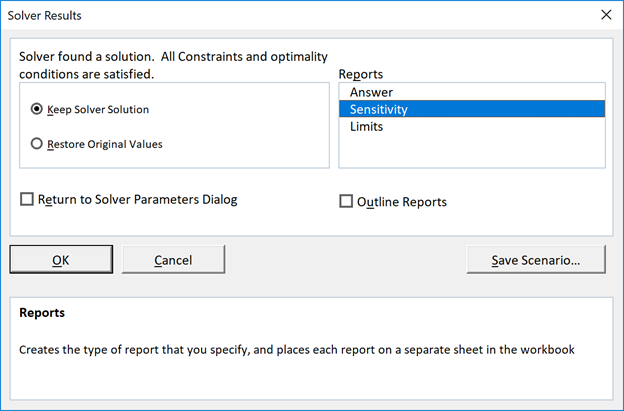
Figure 1: Screenshot of a Solver Results dialog box in Excel
A sensitivity analysis report helps in better understanding the optimal solution and its level of sensitivity to certain problem parameters. Specifically, the sensitivity analysis report provides two sets of measures: (1) sensitivity of the objective function coefficients, and (2) sensitivity of the constraints’ right-hand-side values. This information can potentially be used by decision makers to further improve the objective function value by manipulating/relaxing the values used in the problem definition.
5 Transportation Modeling
The goal of the transportation problem is to minimize the total cost of transportation, where there is shipping of products from several sources (i.e., supply centers such as production plants) to sinks (i.e., demand centers such as warehouses). This shipping is accomplished while complying with supply-and-demand constraints, where the supply constraints limit the amounts of products shipped out of a source (e.g., a production plant or distribution center), and the demand constraints enforce the amounts of products to be sent to each sink (e.g., a warehouse or retail outlet). Figure 2 illustrates this in a simple pictorial representation.
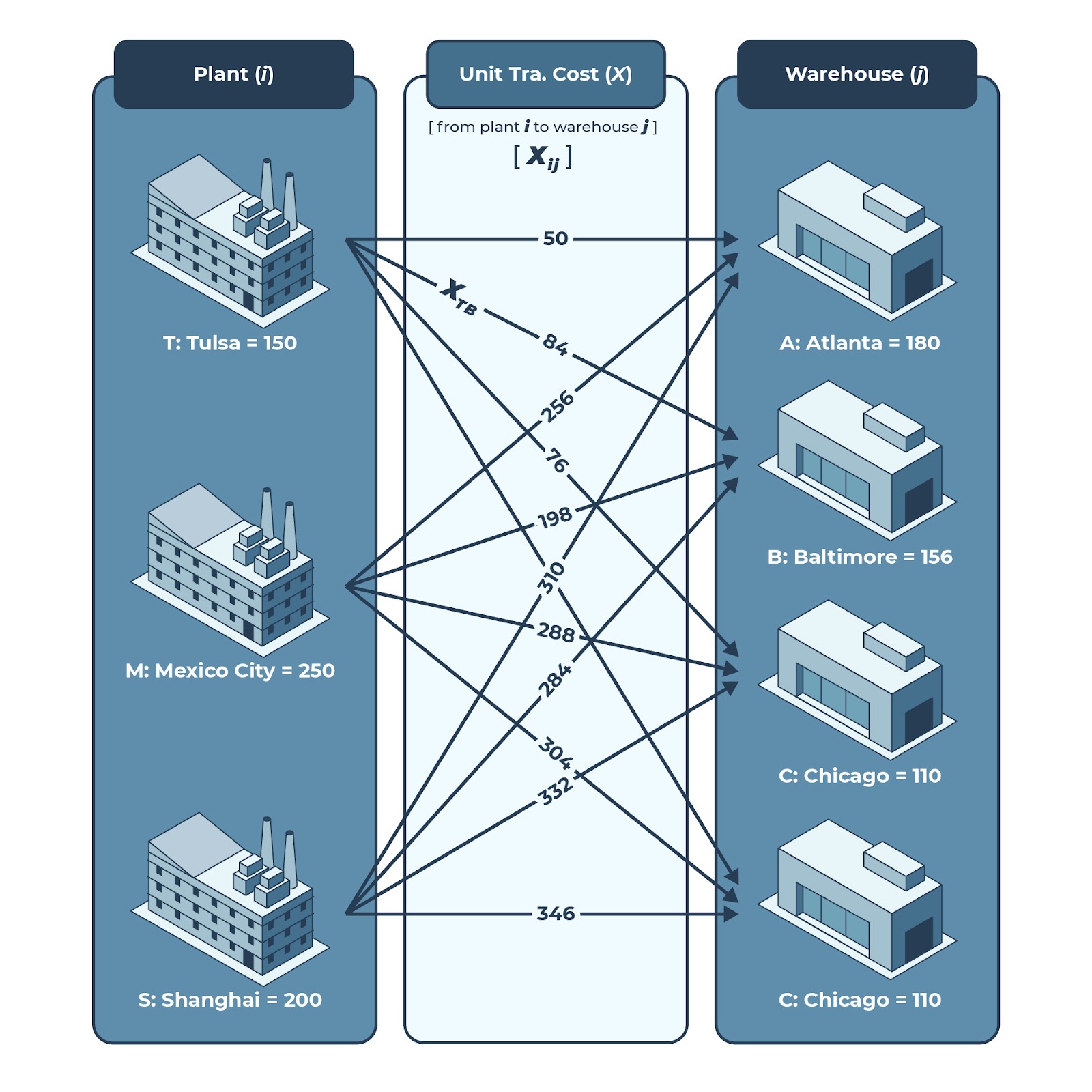
Figure 2: Transportation modeling illustration
In this overly simplified example, we have three sources (i.e., three plants) and four sinks (i.e., four warehouses). Any of these plants can send products to any warehouse, each shipment with a different unit transportation cost. Each plant has production limits and each warehouse has demand requirements. The goal in this example is to find a solution that produces the minimum total transportation cost. This problem can also be represented as a simple matrix as shown in Figure 3 below.
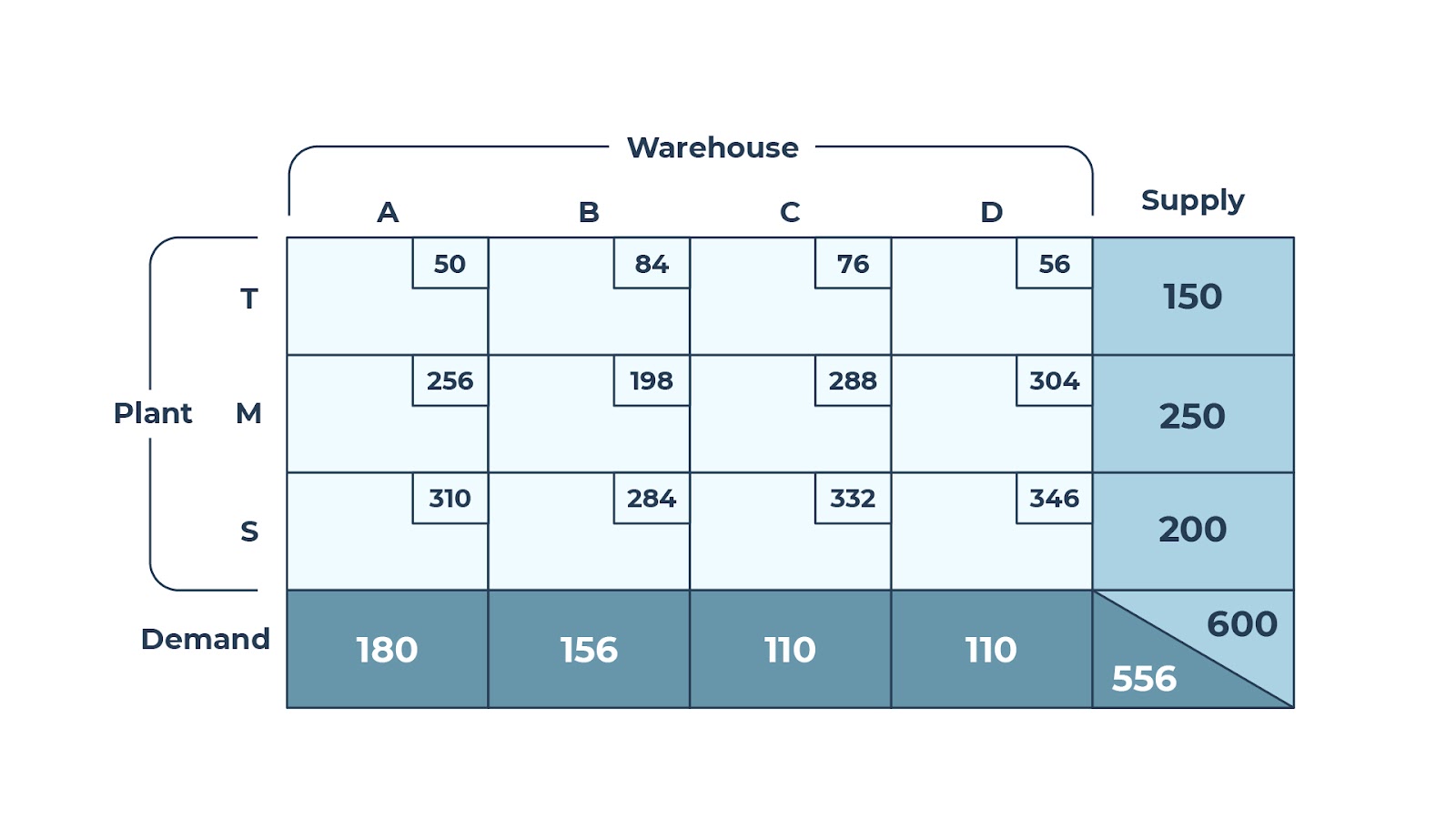
Figure 3: The same transportation model represented as a matrix
This problem can be solved heuristically (using common logic) or optimally (using linear programming). Let’s look at each solution in more detail below.
5.1 Heuristic/Logical Solution
To solve this problem, we can use a common-sense logical rule to assign shipment quantities into 12 decision cells which would minimize the total transportation cost while still complying with the supply-and-demand constraints. A commonly used heuristic is called “maximizing shipment quantities for minimum unit cost options.” In execution of this heuristic, one would find the minimum unit transportation cost cell and assign the largest possible value (quantity on that cell) while complying with the supply-and-demand constraints. This procedure is repeated until all 12 cells are filled with zeros and some non-zero integer numbers. This would produce a good solution but not necessarily the best (i.e., the optimal) solution.
5.2 Optimal/Excel Solution
The same problem can also be solved using Excel Solver, optimally. We can accomplish this in a similar way to that which we followed while solving the product-mix problem, i.e., by formulating the problem in an Excel sheet, specifying the optimization problem parameters in the Solver dialog box, and generating the optimal solution.